
 GPS & GNSS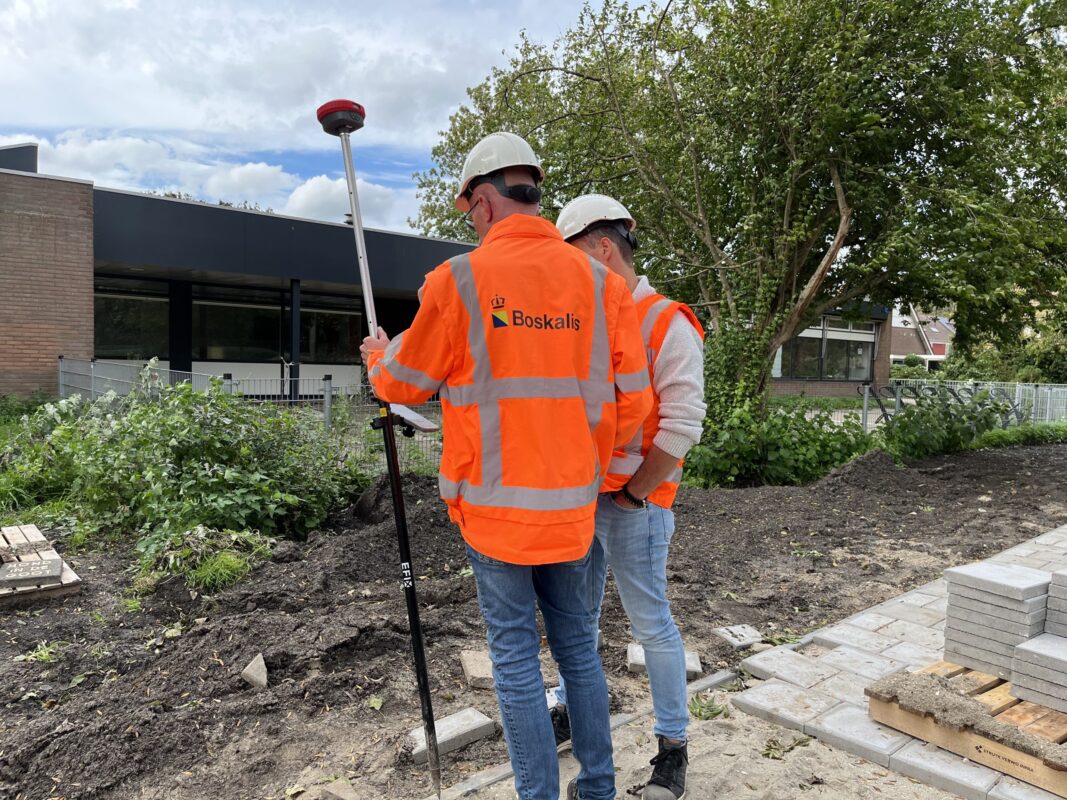
 Lidar scanning
 Total Station
Measure stockpile volumes with EFIX surveying equipment
5 min read
Measure stockpile volumes with EFIX surveying equipment #
This video demonstrates how to collect survey points around a stockpile and calculate its volume using an EFIX GNSS receiver and field controller.
The workflow has three main parts: configure the survey, collect the stockpile points, and create the volume calculation.
Quick summary #
- Open the volumes project and enter Survey.
- Set the survey method to Continuous survey.
- Select Distance 3D and enter a 1 m interval.
- Walk around the stockpile to record and close its boundary.
- Collect additional points across the stockpile surface.
- Open Tools > Volumes and create volume v1.
- Select Stockpile/Pit and Surface to base.
- Create surface s1 using the recorded points and closed boundary.
- Preview the triangulated surface in 2D and 3D.
- Tap Calculate to view the cut-and-fill volumes.
What you need #
- An EFIX GNSS receiver
- A survey pole
- A field controller running the surveying application shown in the video
The exact EFIX receiver model and software version are not readable in the video.
Step 1: Open the survey project #
From the application’s main screen, open the project named volumes.
Tap Survey to enter the point-collection screen.
The status bar shows that the GNSS receiver has a fixed solution before measurements begin.
Step 2: Configure continuous point collection #
On the survey screen, open the settings by tapping the gear icon.
The volumes-Settings page opens on the Survey tab.
Set the following options:
- Survey method: Continuous survey
- Store fixed solutions only: Enabled
- Auto increment name interval: 1
- Mode: Distance 3D
- Distance 3D: 1 m
The video briefly opens the mode list, where the visible options include:
- Time
- Distance 2D
- Distance 2D or delta H
- Distance 3D
After selecting Distance 3D, the distance is changed from 5.000 m to 1 m.
Return to the survey screen.
Step 3: Measure the stockpile boundary #
Start the continuous survey and walk around the outside edge of the stockpile.
Keep the survey pole positioned along the boundary while moving around the stockpile. The application automatically records points according to the selected 1-meter three-dimensional distance interval.
The point number increases as new measurements are stored.
After completing the perimeter, tap the command used to finish the line.
A confirmation message appears:
Close the current polyline?
Tap Yes.
The completed boundary is displayed as a closed line on the map.
Step 4: Measure points across the stockpile surface #
Continue collecting points over the stockpile rather than only around its outside edge.
The operator walks back and forth across the area while holding the survey pole on the surface being measured.
The application displays the measured points and the lines created during collection. By the end of this stage, the survey screen shows approximately 73 recorded points.
The exact walking pattern is not defined by an on-screen instruction, but the video shows measurements being distributed across the full surface inside the boundary.
Step 5: Open the Volumes tool #
Tap the three-dot menu in the upper-right corner.
The application opens the volumes-All menu page.
Open the Tools tab and select Volumes.
The video also shows another menu containing a Volumes shortcut represented by an icon marked with cubic-meter units.
Step 6: Create a new volume calculation #
On the volumes-New a volume page, enter the following settings:
- Name: v1
- Cut swell factor: 1
- Method: Stockpile/Pit
- Calculation direction: Surface to base
The method initially appears as Reference elevation and is then changed to Stockpile/Pit.
The Surface field must be completed before the calculation can run.
Step 7: Create the stockpile surface #
Open the Surface field to create a new surface.
On the volumes-New surface page, enter:
- Name: s1
The remaining sections are:
- Points
- Breaklines
- Boundaries
- Surface style
- Color
Select the measured points #
Open Points.
A menu appears with these options:
- Select from point list
- Select from map
- Range of points
Choose Select from point list.
The volumes-Points page opens. Tap Select all to include the measured survey points, and then tap OK.
The surface page shows 72 points selected. The broader project view previously showed 73 points, so one recorded item may not have been included in the surface selection. The video does not explain the difference.
Select the boundary #
Open Boundaries and select the previously measured closed outline from the map.
The boundary is highlighted. Confirm the selection by tapping the checkmark or OK.
The surface page then shows:
- 72 points
- 0 breaklines
- 1 boundary
Leave Breaklines unselected.
Step 8: Preview and check the surface #
Tap OK to generate the surface preview.
The volumes-Preview page opens in 2D view. The measured points and triangulated surface are shown inside the selected boundary.
Tap 3D to inspect the surface as a three-dimensional model.
The vertical toolbar contains tools for examining and editing the triangulation. The video displays an editing option labeled Delete Triangle, although it does not clearly confirm that a triangle is deleted.
Rotate or inspect the model as needed, and then tap OK.
Step 9: Calculate the volume #
The application returns to the volume setup page.
Confirm that the settings show:
- Name: v1
- Cut swell factor: 1
- Method: Stockpile/Pit
- Surface: s1
- Calculation direction: Surface to base
Tap Calculate.
Result #
The volumes-Result page opens.
The Details tab displays:
- Project: volumes
- Name: v1
- Date: 05-06-25 16:55:54
- Method: Stockpile/Pit
- Calculation direction: Surface to base
- Surface: s1
- Cut swell factor: 1.000
The View tab displays the calculated surface model and the volume results:
- Fill: 0.010 cubic meters
- Cut: 10.878 cubic meters
An Export Report button is available at the bottom of the result page.
 GPS & GNSS
 Total Stations
 Data collectors
 Software
 Correction services
 Machine control
 External radio
 Lasers & levellers
 Marine
 Accessories